Gaussian Naive Bayes is a popular algorithm for classification tasks, especially for problems involving continuous numerical data. This blog will discuss implementing multiclass Classification using Gaussian Naive Bayes through a vectorization approach, which is much faster than the for-loop approach.

We will start with the basics of Bayes’ Theorem, Gaussian distribution and Naive Bayes. In the second section, we’ll implement Gaussian Naive Bayes using Python from scratch. However, we’ll use Numpy for certain operations but not libraries like sklearn to implement the prediction function. We’ll only use sklearn for splitting, encoding the dataset and evaluating the model.

Link complete code for the Implementation —

Bayes’ Theorem

Bayes Theorem tells us the Probability of an event happening (Y) given some observed evidence (X).

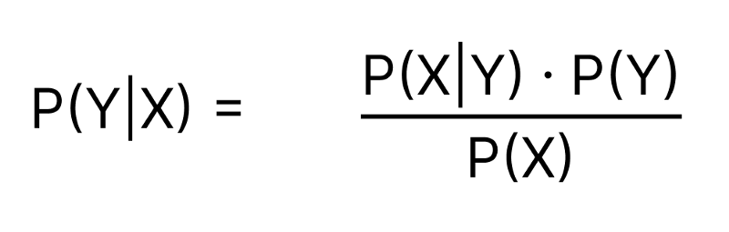
P(Y|X): Conditional Probability of Y given X is observed

P(X|Y): Likelihood of X being observed given that Y occurred

P(Y): Prior Probability of event Y

P(X): Prior Probability of evidence X

If you want a better intuition behind the Bayes Theorem, I would suggest reading this article: Bayes’ Theorem with Lego.

Gaussian Distribution Function

Gaussian distribution, also known as Normal distribution, is a probability distribution commonly used to describe natural phenomena such as height or weight distribution in a population, measurement errors, and several other phenomena. It is naturally occurring in many real-world situations.

In a Gaussian distribution, the Probability of x is given by:

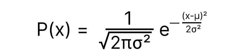
σ² = Variance = (Standard Deviation)²

µ = Mean

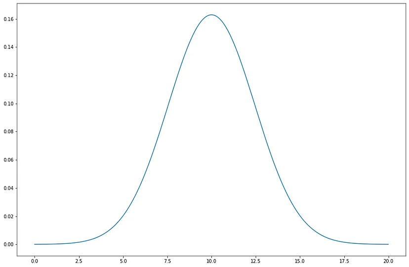
Fig: A Gaussian distribution with μ = 10 and σ² = 6

Naive Bayes

Naive Bayes is a classification algorithm based on Bayes’ Theorem with a ‘naive’ assumption that features of the dataset are independent of Each other.

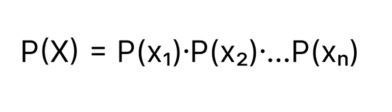
Let’s say our dataset has n features ( x₁, x₂…, xₙ). We assume the features x₁, x₂, x₃ are independent, then Probability of an event X = {x₁, x₂…, xₙ}

Formula for P(Y = y | X = {x₁, x₂…, xₙ}) can be expanded to

---

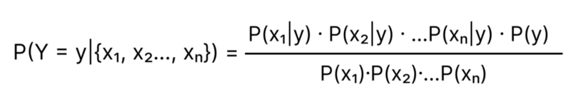
Implementing Gaussian Naive Bayes Classifier

Gaussian Naive Bayes is a variation of Naive Bayes that assumes that data follows a Gaussian distribution.

We will use the famous Iris Dataset for this article. It consists of 50 examples for each label, each with four different features.

Let’s take a look at our data.

Few selected values from the Iris Dataset

Using the code snippet below, you can import the Iris Dataset directly from the UCI ML repository.

df = pd.read_csv('https://archive.ics.uci.edu/ml/machine-learning-databases/iris/iris.data',
                 sep=',',
                 names = ['sepal length','sepal width','petal length','petal width','class']
                 )

Visualizing out data

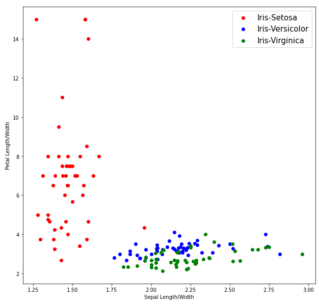
We can see from the above plots that Iris-Setosa is linearly separable from the other two, but the other two are not linearly separable.

Encoding Labels and Splitting Dataset into Test and Training set

Encoding Labels

# Separating the Labels into a numpy array
Y = np.asarray(df['class'])

# Encoding Labels using Scikit-Learn LabelEncoder  
from sklearn.preprocessing import LabelEncoder  
le = LabelEncoder()  
Y = le.fit_transform(Y)

Splitting the dataset into a Test set and Training Set

#splitting the data into training and testing sets using Scikit-Learn
from sklearn.model_selection import train_test_split  
x_train, x_test, y_train, y_test = train_test_split(df, Y, test_size = 0.2, random_state = 5, stratify=Y)

# stratify=Y evenly distributes target labels in training and test set  
# randome_state = n controls the shuffling process, setting random state to a certain values makes the splitting deterministic

Here I chose NOT to drop the target labels from x_train because it will help calculate the mean and variance of subgroups later. We can drop it before making predictions from the test set (or training set).

Calculating required variables

Calculating Prior Probability of classes

m = x_train.shape[0]  
label_counts = x_train['class'].value_counts()  
prior_y = np.array(label_counts)/m

We get the prior Probability of all labels as a 1-D numpy vector.

Calculating the Mean and Variance of different subgroups

# calculating Mean and Variance of Features grouped by class labels

mean_values = x_train.groupby('class')[['sepal length', 'sepal width','petal length','petal width']].mean()  
var_values = x_train.groupby('class')[['sepal length', 'sepal width','petal length','petal width']].var()

# Conveting Pandas Datafram into 2-D Numpy Matrix  
means = np.asarray(mean_values)  
vars = np.asarray(var_values)

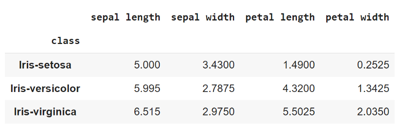
mean-values of features grouped by class

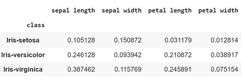
the variance of features grouped by class

Gaussian Probability Function

def gaussian_probability(x,mu, sigma2):  
a = (1/np.sqrt(2*np.pi*sigma2))  
b = np.exp(-np.square(x-mu)/(2*sigma2))  
return a*b

Prediction Function

We ignore the denominator of the Bayes Formula since it’s the same across all probabilities of all labels. Hence, we can calculate and compare P(X|y) for all labels.

def predict(test_data):  
    """  
    test_data ndarray(4,)  
    """  

    # PX_y = P(X|y)  
    # Py_X = P(y|X)  

    PX_y = gaussian_probability(test_data,means,vars) #step -1  
    PX_y = np.prod(PX_y,axis=1) #step - 2  
    Py_X = PX_y*prior_y #step - 3  

    return np.argmax(Py_X)

In step — 1, On passing test_data, which is a vector of size 4 to the gaussian_probability function, It is broadcasted into a matrix of size 3x4 such that each row of the matrix holds vector test_data. gaussian_probability function returns a 3x4 matrix. Every value in the matrix is calculated using values at corresponding positions in broadcasted test_data matrix, means and vars matrix.

PX_y after step- 1

In step — 2, the Product is calculated along each row of the PX_y matrix and saved into a vector of size 3.

PX_y is now a vector containing the likelihood probability of observing features X given y for all labels.

In step — 3, We get Py_X, i.e. P(y|X) as the Product of PX_y and prior_y. Py_X contains relative values of probabilities of all labels. They are not actual probabilities but can be used to compare the probabilities of different classes.

Note: values stored in Py_X are not actual probabilities because we’ve ignored the denominator during our calculation.

The index of the maximum value in Py_X represents the class that has the maximum probability among all the classes. We return the index of the maximum value in Py_X as the prediction.

This is it. Good Luck coding.

---

For any queries, you can reach out to me via Twitter @priyanshh32 or patidarpriyansh936@gmail.com